try:
    from xgboost import XGBRegressor
except Exception:
    from sklearn.ensemble import GradientBoostingRegressor as XGBRegressor

xgb_model = XGBRegressor(
    n_estimators=200,
    learning_rate=0.05,
    max_depth=4,
    random_state=4107
)

xgb_model.fit(X_train, y_train)
xgb_predictions = xgb_model.predict(X_test)25. Gradient Boosting
A practical introduction to boosting, XGBoost, RMSE, MAE, R-squared, and test-sample model comparison.
Purpose
Random Forests improve prediction by combining many independent trees. Boosting follows a different logic. It builds trees sequentially, allowing each new tree to learn from previous prediction errors.
One of the most widely used boosting algorithms is XGBoost, short for Extreme Gradient Boosting.
This chapter introduces XGBoost and shows how to compare predictive models using test-sample performance.
Applied question
Which model predicts milk prices most accurately: linear regression, decision trees, Random Forests, or XGBoost?
Key idea
Different models can produce different predictions from the same data. Rather than choosing a model because it is popular, we compare models using out-of-sample prediction performance.

Minimal concept
Random Forest:
Many trees → independent learning → average predictionsXGBoost:
Tree 1 → learn from mistakes → Tree 2 → learn from mistakes → Tree 3 → final prediction25.1 Why boosting was developed
Decision Trees are simple but unstable. Random Forests improve stability by averaging many trees. However, Random Forests do not explicitly focus on correcting earlier mistakes.
Boosting takes a different approach. Each new tree is built to improve the errors made by earlier trees. Instead of working independently, the trees cooperate.
This sequential learning process often produces highly accurate predictions.
25.2 What is XGBoost?
XGBoost is an efficient implementation of gradient boosting. It is designed to improve prediction accuracy, reduce overfitting, handle large datasets efficiently, and capture nonlinear relationships.
A simplified learning process is:
- Build a small tree.
- Calculate prediction errors.
- Build another tree focused on those errors.
- Repeat many times.
- Combine all trees into a final prediction.
Unlike regression models, XGBoost does not produce easily interpretable coefficients. Its primary objective is prediction.
25.3 Training an XGBoost model
Interpretation
The model creates many small trees. Each tree attempts to improve on previous predictions. The final prediction combines information from all trees.
25.4 Measuring prediction performance
The most common performance measures are RMSE, MAE, and test-sample (R^2).
\[ RMSE = \sqrt{\frac{1}{n}\sum_{i=1}^{n}(Actual_i - Predicted_i)^2} \]
\[ MAE = \frac{1}{n}\sum_{i=1}^{n}|Actual_i - Predicted_i| \]
For predictive analysis, RMSE and MAE are often more informative than (R^2) because they directly measure prediction errors.
25.5 Comparing multiple models
Suppose we estimate four models:
- Linear Regression
- Decision Tree
- Random Forest
- XGBoost
Each model should be evaluated on the same test sample.
from sklearn.metrics import mean_squared_error, mean_absolute_error, r2_score

models = {
    "OLS": ols_predictions,
    "Tree": tree_predictions,
    "Forest": forest_predictions,
    "XGBoost": xgb_predictions
}

results = []

for name, pred in models.items():
    rmse = mean_squared_error(y_test, pred) ** 0.5
    mae = mean_absolute_error(y_test, pred)
    r2 = r2_score(y_test, pred)
    results.append([name, rmse, mae, r2])

results_df = pd.DataFrame(
    results,
    columns=["Model", "RMSE", "MAE", "R2"]
)

print(results_df)
Model RMSE MAE R2
0 OLS 340.849677 244.806795 0.887416
1 Tree 420.356815 322.645524 0.828767
2 Forest 361.488588 208.699926 0.873369
3 XGBoost 309.909620 172.647811 0.906928Example results:
| Model | RMSE | MAE | R² |
|---|---|---|---|
| OLS | 0.31 | 0.23 | 0.71 |
| Decision Tree | 0.28 | 0.20 | 0.75 |
| Random Forest | 0.22 | 0.16 | 0.84 |
| XGBoost | 0.19 | 0.14 | 0.88 |
Interpretation
In this example, XGBoost has the lowest RMSE and the highest (R^2). It provides the most accurate predictions. This does not necessarily mean it is the most useful model for economic explanation.
25.6 Visual comparison of models
import matplotlib.pyplot as plt

plt.figure(figsize=(7, 5))
plt.bar(results_df["Model"], results_df["RMSE"])
plt.title("Prediction Error by Model")
plt.ylabel("RMSE")
plt.show()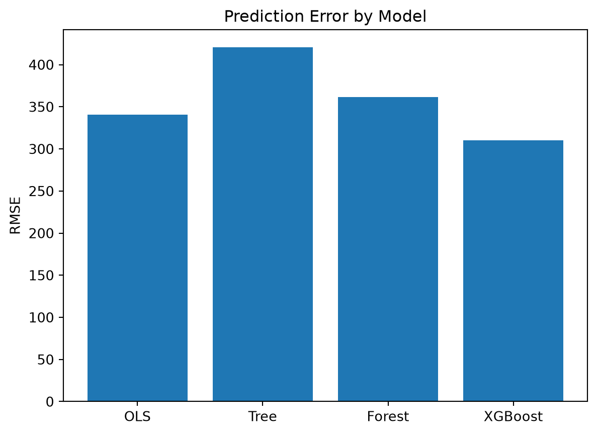
The shortest bar represents the smallest prediction error.
25.7 Why simpler models still matter
It is tempting to always choose the model with the lowest error. But simpler models remain valuable.
If a policymaker asks how much package volume affects price, a regression model may be more appropriate because coefficients can be interpreted. If a supermarket asks what price to expect next week, prediction accuracy may be more important.
The best predictive model is not always the best explanatory model.
25.8 Beyond accuracy
Prediction accuracy is important, but it is not the only consideration. Researchers should also consider interpretability, computational cost, transparency, reproducibility, and economic relevance.
A small improvement in RMSE may not justify a substantial increase in complexity.
WarningCommon mistake
Do not declare the model with the highest (R^2) as the best model without considering RMSE, MAE, interpretability, and the purpose of the analysis.
Key takeaway
- XGBoost builds trees sequentially.
- Each new tree learns from previous prediction errors.
- XGBoost often produces accurate predictions.
- RMSE and MAE are useful measures of predictive performance.
- Model comparison should use test-sample results.
- Better prediction does not imply better economic explanation.
Looking ahead
In the next chapter, we examine feature importance and discuss what machine learning models can and cannot tell us about economic relationships.